University of Florida/Egm6321/f12.Rep5hid

${\displaystyle \displaystyle \mathbf {A} \in \mathbb {R} ^{(n\times n)}}$

and

${\displaystyle {\underset {\color {red}n\times n}{\exp[\mathbf {A} ]}}={\underset {\color {red}n\times n}{\mathbf {I} }}+{\underset {\color {red}n\times n}{{\frac {1}{1!}}\mathbf {A} }}+{\underset {\color {red}n\times n}{{\frac {1}{2!}}\mathbf {A} ^{2}}}+....={\underset {\color {red}n\times n}{\sum _{k=0}^{\infty }{\frac {1}{k!}}\mathbf {A} ^{k}}}}$

(Eq.(2)p.20-2b)

${\displaystyle \displaystyle \exp \mathbf {A} ^{T}=(\exp \mathbf {A} )^{T}}$

(Eq.5.1.1)

We will first expand the LHS, then the RHS of (Eq. 5.1.1) using (Eq.(2)p.20-2b) and compare the two expressions.

Expanding the LHS,

${\displaystyle {\underset {\color {red}n\times n}{\exp[\mathbf {A^{T}} ]}}={\underset {\color {red}n\times n}{\mathbf {I^{T}} }}+{\underset {\color {red}n\times n}{{\frac {1}{1!}}\mathbf {A^{T}} }}+{\underset {\color {red}n\times n}{{\frac {1}{2!}}[\mathbf {A^{T}} ]^{2}}}+....={\underset {\color {red}n\times n}{\sum _{k=0}^{\infty }{\frac {1}{k!}}\mathbf {[} {A^{T}}]^{k}}}}$

But we know that

${\displaystyle \mathbf {I} ^{T}=\mathbf {I} }$

${\displaystyle \therefore {\underset {\color {red}n\times n}{\exp[\mathbf {A^{T}} ]}}={\underset {\color {red}n\times n}{\mathbf {I} }}+{\underset {\color {red}n\times n}{{\frac {1}{1!}}\mathbf {A^{T}} }}+{\underset {\color {red}n\times n}{{\frac {1}{2!}}[\mathbf {A^{T}} ]^{2}}}+....={\underset {\color {red}n\times n}{\sum _{k=0}^{\infty }{\frac {1}{k!}}\mathbf {[} {A^{T}}]^{k}}}}$

(Eq.5.1.2)

Now expanding the RHS,

${\displaystyle {\underset {\color {red}n\times n}{\exp[\mathbf {A} ]^{T}}}=\left[{\underset {\color {red}n\times n}{\mathbf {I} }}+{\underset {\color {red}n\times n}{{\frac {1}{1!}}\mathbf {A} }}+{\underset {\color {red}n\times n}{{\frac {1}{2!}}[\mathbf {A} ]^{2}}}+....={\underset {\color {red}n\times n}{\sum _{k=0}^{\infty }{\frac {1}{k!}}\mathbf {[} {A}]^{k}}}\right]^{T}}$

Which on calculating, reduces to

${\displaystyle {\underset {\color {red}n\times n}{\exp[\mathbf {A^{T}} ]}}={\underset {\color {red}n\times n}{\mathbf {I^{T}} }}+{\underset {\color {red}n\times n}{{\frac {1}{1!}}\mathbf {A^{T}} }}+{\underset {\color {red}n\times n}{{\frac {1}{2!}}[\mathbf {A^{T}} ]^{2}}}+....={\underset {\color {red}n\times n}{\sum _{k=0}^{\infty }{\frac {1}{k!}}\mathbf {[} {A^{T}}]^{k}}}}$

or

${\displaystyle {\underset {\color {red}n\times n}{\exp[\mathbf {A^{T}} ]}}={\underset {\color {red}n\times n}{\mathbf {I} }}+{\underset {\color {red}n\times n}{{\frac {1}{1!}}\mathbf {A^{T}} }}+{\underset {\color {red}n\times n}{{\frac {1}{2!}}[\mathbf {A^{T}} ]^{2}}}+....={\underset {\color {red}n\times n}{\sum _{k=0}^{\infty }{\frac {1}{k!}}\mathbf {[} {A^{T}}]^{k}}}}$

(Eq.5.1.3)

Comparing (Eq. 5.1.2) and (Eq. 5.1.3)

We conclude the LHS = RHS, Hence Proved.

A Diagonal Matrix

${\displaystyle \displaystyle \mathbf {D} ={\text{Diag}}[d_{1},d_{2},d_{3},....,d_{n}]}$, where, ${\displaystyle \mathbf {D} \in \mathbb {C} ^{n\times n}}$.

(Eq.(2)p.20-2b)

Show that

${\displaystyle \displaystyle \exp[\mathbf {D} ]={\text{Diag}}[e^{d_{1}},e^{d_{2}},e^{d_{3}},....,e^{d_{n}}]}$, where, ${\displaystyle \exp[\mathbf {D} ]\in \mathbb {C} ^{n\times n}}$.

(Eq.(3)p.20-2b)

We know, from Lecture Notes ^[3],

${\displaystyle {\underset {\color {red}n\times n}{\exp[\mathbf {A} ]}}={\underset {\color {red}n\times n}{\mathbf {I} }}+{\underset {\color {red}n\times n}{{\frac {1}{1!}}\mathbf {A} }}+{\underset {\color {red}n\times n}{{\frac {1}{2!}}\mathbf {A} ^{2}}}+....={\underset {\color {red}n\times n}{\sum _{k=0}^{\infty }{\frac {1}{k!}}\mathbf {A} ^{k}}}}$

(Eq.(2)p.15-3)

Let us consider a Simple yet Generic 4x4 Complex Diagonal Matrix ${\displaystyle \mathbf {D} }$

${\displaystyle \mathbf {D} ={\begin{bmatrix}ai&0&0&0\\0&bi&0&0\\0&0&ci&0\\0&0&0&di\end{bmatrix}}}$

(Eq.5.2.2)

where ${\displaystyle i={\sqrt {-1}}}$.

Applying (Eq.(2)p.15-3) to (Eq.5.2.2) and expanding,

${\displaystyle \exp[\mathbf {D} ]=\underbrace {\begin{bmatrix}1&0&0&0\\0&1&0&0\\0&0&1&0\\0&0&0&1\end{bmatrix}} _{\color {blue}{\text{Matrix 1}}}+{\frac {1}{1!}}\underbrace {\begin{bmatrix}ai&0&0&0\\0&bi&0&0\\0&0&ci&0\\0&0&0&di\end{bmatrix}} _{\color {blue}{\text{Matrix 2}}}+{\frac {1}{2!}}\underbrace {{\begin{bmatrix}ai&0&0&0\\0&bi&0&0\\0&0&ci&0\\0&0&0&di\end{bmatrix}}*{\begin{bmatrix}ai&0&0&0\\0&bi&0&0\\0&0&ci&0\\0&0&0&di\end{bmatrix}}} _{\color {blue}{\text{Matrix 3}}}+\ldots +{\frac {1}{k!}}\underbrace {{\begin{bmatrix}ai&0&0&0\\0&bi&0&0\\0&0&ci&0\\0&0&0&di\end{bmatrix}}*\ldots *{\begin{bmatrix}ai&0&0&0\\0&bi&0&0\\0&0&ci&0\\0&0&0&di\end{bmatrix}}} _{\color {blue}{\text{multiply k times - Matrix k}}}}$

(Eq.5.2.3)

Simplifying Term 2 and other higher power terms (upto Term k) in the following way,

${\displaystyle {\text{Matrix 3}}={\begin{bmatrix}ai&0&0&0\\0&bi&0&0\\0&0&ci&0\\0&0&0&di\end{bmatrix}}*{\begin{bmatrix}ai&0&0&0\\0&bi&0&0\\0&0&ci&0\\0&0&0&di\end{bmatrix}}}$

${\displaystyle {\text{Matrix 3}}={\begin{bmatrix}(ai)^{2}&0&0&0\\0&(bi)^{2}&0&0\\0&0&(ci)^{2}&0\\0&0&0&(di)^{2}\end{bmatrix}}}$

(Eq.5.2.4)

Similarly,

${\displaystyle {\text{Matrix k}}={\begin{bmatrix}(ai)^{k}&0&0&0\\0&(bi)^{k}&0&0\\0&0&(ci)^{k}&0\\0&0&0&(di)^{k}\end{bmatrix}}}$

(Eq.5.2.5)

Using (Eq.5.2.4) and (Eq.5.2.5) in (Eq.5.2.3) and carrying out simple matrix addition, we get,

${\displaystyle exp[\mathbf {D} ]={\begin{bmatrix}(1+{\frac {1}{1!}}(ai)+{\frac {1}{2!}}(ai)^{2}+\ldots +{\frac {1}{k!}}(ai)^{k}&0&0&0\\0&(1+{\frac {1}{1!}}(bi)+{\frac {1}{2!}}(bi)^{2}+\ldots +{\frac {1}{k!}}(bi)^{k})&0&0\\0&0&(1+{\frac {1}{1!}}(ci)+{\frac {1}{2!}}(ci)^{2}+\ldots +{\frac {1}{k!}}(ci)^{k})&0\\0&0&0&(1+{\frac {1}{1!}}(di)+{\frac {1}{2!}}(di)^{2}+\ldots +{\frac {1}{k!}}(di)^{k})\end{bmatrix}}}$

(Eq.5.2.6)

But every diagonal term of the matrix is of the form,

${\displaystyle \exp(x)=1+{\frac {1}{1!}}x+{\frac {1}{2!}}x^{2}+\ldots +{\frac {1}{n!}}x^{n}}$

(Eq.5.2.7)

Therefore, (Eq.5.2.6) can be rewritten as,

${\displaystyle exp[\mathbf {D} ]={\begin{bmatrix}exp(ai)&0&0&0\\0&exp(bi)&0&0\\0&0&exp(ci)&0\\0&0&0&exp(di)\end{bmatrix}}={\begin{bmatrix}e^{ai}&0&0&0\\0&e^{bi}&0&0\\0&0&e^{ci}&0\\0&0&0&e^{di}\end{bmatrix}}}$

(Eq.5.2.8)

${\displaystyle {\text{(ai)}},{\text{(bi)}},{\text{(ci)}},{\text{(di)}}}$ are nothing but the diagonal elements of the original matrix in (Eq.5.2.2). Hence,

${\displaystyle \displaystyle \exp[\mathbf {D} ]={\text{Diag}}[e^{d_{1}},e^{d_{2}},e^{d_{3}},e^{d_{4}}]}$

(Eq.5.2.9)

Similarly it can be easily found for an ${\displaystyle n\times n}$ complex diagonal matrix that

${\displaystyle \displaystyle \exp[\mathbf {D} ]={\text{Diag}}[e^{d_{1}},e^{d_{2}},e^{d_{3}},....,e^{d_{n}}]}$

(Eq.5.2.10)

Hence Proved.

A matrix ${\displaystyle \mathbf {A} }$ can be decomposed as

${\displaystyle \displaystyle \mathbf {A} =\mathbf {\Phi } \,\mathbf {\Lambda } \,\mathbf {\Phi } ^{-1}}$

(Eq.(2) p.20-4)

where

${\displaystyle \mathbf {\Lambda } }$ is the diagonal matrix of eigenvalues of matrix ${\displaystyle \mathbf {A} }$

${\displaystyle \displaystyle \mathbf {\Lambda } ={\text{Diag}}[\lambda _{1},\lambda _{2},\ldots ,d_{n}]\in \mathbb {C} ^{n\times n}}$

(Eq.(5) p.20-3)

and

${\displaystyle \mathbf {\Phi } }$ is the matrix established by n linearly independent eigenvectors ${\displaystyle {\boldsymbol {\phi }}_{i}(i=1,2,3,\ldots ,n)}$of matrix ${\displaystyle \mathbf {A} }$, that is,

${\displaystyle \displaystyle \mathbf {\Phi } =[{\boldsymbol {\phi }}_{1},{\boldsymbol {\phi }}_{2},\ldots ,{\boldsymbol {\phi }}_{n}]\in \mathbb {C} ^{n\times n}}$

(Eq.(2) p.20-3)

Show that

${\displaystyle \displaystyle \exp[\mathbf {A} ]=\mathbf {\Phi } \,{\text{Diag}}[\,e^{\lambda _{1}},\,e^{\lambda _{2}},\ldots ,\,e^{\lambda _{n}}]\mathbf {\Phi } ^{-1}}$

The power series expansion of exponentiation of matrix ${\displaystyle \mathbf {A} }$ in terms of that matrix has been given as

${\displaystyle \displaystyle \exp[\mathbf {A} ]=\mathbf {I} +{\frac {1}{1!}}\mathbf {A} +{\frac {1}{2!}}\mathbf {A} ^{2}+{\frac {1}{3!}}\mathbf {A} ^{3}+\cdots =\sum _{k=0}^{\infty }{\frac {1}{k!}}\mathbf {A} ^{k}}$

(Eq.(2) p.15-3)

Since matrix ${\displaystyle \mathbf {A} }$ can be decomposed as,

${\displaystyle \displaystyle \mathbf {A} =\mathbf {\Phi } \,\mathbf {\Lambda } \,\mathbf {\Phi } ^{-1}}$

(Eq.(2) p.20-4)

Expanding the ${\displaystyle k}$ power of matrix ${\displaystyle \mathbf {A} }$ yields

${\displaystyle \displaystyle \mathbf {A} ^{k}=\underbrace {(\mathbf {\Phi } \,\mathbf {\Lambda } \,\mathbf {\Phi } ^{-1})(\mathbf {\Phi } \,\mathbf {\Lambda } \,\mathbf {\Phi } ^{-1})\cdots (\mathbf {\Phi } \,\mathbf {\Lambda } \,\mathbf {\Phi } ^{-1})} _{{\text{number of factors}}(\mathbf {\Phi } \,\mathbf {\Lambda } \,\mathbf {\Phi } ^{-1}){\text{is k}}}}$

(Eq.5.3.1)

Where the factors ${\displaystyle (\mathbf {\Phi } )}$ which are neighbors of factors ${\displaystyle (\mathbf {\Phi } ^{-1})}$ can be all cancelled in pairs, that is,

${\displaystyle \displaystyle \mathbf {A} ^{k}=\mathbf {\Phi } \,\mathbf {\Lambda } \,{\cancelto {\mathbf {I} }{\mathbf {\Phi } ^{-1}\mathbf {\Phi } \,}}\mathbf {\Lambda } \,{\cancelto {\mathbf {I} }{\mathbf {\Phi } ^{-1}\mathbf {\Phi } \,}}\mathbf {\Lambda } \,\cdots \mathbf {\Lambda } \,{\cancelto {\mathbf {I} }{\mathbf {\Phi } ^{-1}\mathbf {\Phi } \,}}\,\mathbf {\Lambda } \,\mathbf {\Phi } ^{-1}}$

(Eq.5.3.2)

${\displaystyle \displaystyle \Rightarrow \mathbf {A} ^{k}=\mathbf {\Phi } \,\underbrace {\mathbf {\Lambda } \,\mathbf {\Lambda } \,\mathbf {\Lambda } \,\cdots \mathbf {\Lambda } \,\mathbf {\Lambda } \,} _{{\text{k}}\mathbf {\Lambda } {\text{s}}}\mathbf {\Phi } ^{-1}}$

(Eq.5.3.3)

${\displaystyle \displaystyle \Rightarrow \mathbf {A} ^{k}=\mathbf {\Phi } \,\mathbf {\Lambda } ^{k}\mathbf {\Phi } ^{-1}}$

(Eq.5.3.4)

Thus, the equation (Eq. 5.3.1) can be expressed as

${\displaystyle \displaystyle \exp[\mathbf {A} ]=\sum _{k=0}^{\infty }{\frac {1}{k!}}[\mathbf {A} ^{k}]=\sum _{k=0}^{\infty }{\frac {1}{k!}}[\mathbf {\Phi } \,\mathbf {\Lambda } ^{k}\mathbf {\Phi } ^{-1}]}$

(Eq.5.3.5)

${\displaystyle \displaystyle \Rightarrow \exp[\mathbf {A} ]=\mathbf {\Phi } \,\sum _{k=0}^{\infty }{\frac {1}{k!}}[\mathbf {\Lambda } ^{k}]\mathbf {\Phi } ^{-1}}$

(Eq.5.3.6)

According to the equation (Eq.(2) p.15-3), now we have,

${\displaystyle \displaystyle \exp[\mathbf {A} ]=\mathbf {\Phi } \,\exp[\mathbf {\Lambda } ]\mathbf {\Phi } ^{-1}}$

(Eq.5.3.7)

Referring to the conclusion obtained in R5.2, which is

${\displaystyle \displaystyle \exp[\mathbf {D} ]={\text{Diag}}[\,e^{d_{1}},\,e^{d_{2}},\ldots ,\,e^{d_{n}}]}$

(Eq.(3) p.20-2b)

Replacing the matrix ${\displaystyle \mathbf {D} }$ with ${\displaystyle \mathbf {\Lambda } }$, the elements ${\displaystyle d_{i}}$ with ${\displaystyle \lambda _{i}}$,where ${\displaystyle i=1,2,3,\ldots ,n}$ and then substituting into (Eq. 5.3.7) yields

${\displaystyle \displaystyle \exp[\mathbf {A} ]=\mathbf {\Phi } \,{\text{Diag}}[\,e^{\lambda _{1}},\,e^{\lambda _{2}},\ldots ,\,e^{\lambda _{n}}]\mathbf {\Phi } ^{-1}}$

(Eq.5.3.8)

Exponentiation of a matrix ${\displaystyle \mathbf {A} }$ can be decomposed as

${\displaystyle \displaystyle \exp[\mathbf {A} ]=\mathbf {\Phi } \,{\text{Diag}}[\,e^{\lambda _{1}},\,e^{\lambda _{2}},\ldots ,\,e^{\lambda _{n}}]\mathbf {\Phi } ^{-1}}$

(Eq.(3) p.20-4)

The matrix ${\displaystyle \mathbf {B} }$ is defined in lecture note

${\displaystyle \displaystyle \mathbf {B} ={\begin{bmatrix}0&-1\\1&0\end{bmatrix}}}$

(Eq.(1) p.20-2)

Show

${\displaystyle \displaystyle \mathbf {B} t={\begin{bmatrix}1&1\\-i&i\end{bmatrix}}{\begin{bmatrix}{it}&0\\0&{-it}\end{bmatrix}}{\begin{bmatrix}i&-1\\i&1\end{bmatrix}}{\frac {1}{2i}}}$

(Eq.(1) p.20-5)

and

${\displaystyle \displaystyle \displaystyle \exp[\mathbf {B} t]={\begin{bmatrix}\cos t&-\sin t\\\sin t&\cos t\end{bmatrix}}\neq {\begin{bmatrix}1&e^{-t}\\e^{t}&1\end{bmatrix}}}$

(Eq.(2) p.20-5)

To show the equation (Eq.(1) p.20-5), we should first find eigenvalues ${\displaystyle \lambda }$ of matrix ${\displaystyle \mathbf {B} }$ using the matrix equation as follow, indroduce ${\displaystyle \mathbf {I} }$ to represent Identity matrix.

${\displaystyle \displaystyle f(x)=\left|\lambda \mathbf {I} -\mathbf {B} \right|=0}$

${\displaystyle \displaystyle \Rightarrow f(x)=\left|{\begin{bmatrix}\lambda &0\\0&\lambda \end{bmatrix}}-{\begin{bmatrix}0&-1\\1&0\end{bmatrix}}\right|=\left|{\begin{bmatrix}\lambda &1\\-1&\lambda \end{bmatrix}}\right|=0}$

${\displaystyle \displaystyle \Rightarrow f(x)=\lambda ^{2}+1=0}$

${\displaystyle \displaystyle \Rightarrow \lambda _{1}=i,\lambda _{2}=-i}$

Since the two eigenvalues of matrix ${\displaystyle \mathbf {B} }$ are both obtained, now solve for the corresponding two eigenvectors.

${\displaystyle \displaystyle (\lambda _{1}\mathbf {I} -\mathbf {B} )\mathbf {X} =\mathbf {O} }$

${\displaystyle \displaystyle \Rightarrow ({\begin{bmatrix}\lambda _{1}&0\\0&\lambda _{1}\end{bmatrix}}-{\begin{bmatrix}0&-1\\1&0\end{bmatrix}}){\begin{bmatrix}x_{1}\\x_{2}\end{bmatrix}}={\begin{bmatrix}0\\0\end{bmatrix}}}$

${\displaystyle \displaystyle \Rightarrow {\begin{bmatrix}\lambda _{1}&1\\-1&\lambda _{1}\end{bmatrix}}{\begin{bmatrix}x_{1}\\x_{2}\end{bmatrix}}={\begin{bmatrix}0\\0\end{bmatrix}}}$

(Eq.5.4.1)

Thus, for the first value of ${\displaystyle \lambda }$, we have

${\displaystyle \displaystyle \left\{{\begin{matrix}\lambda _{1}x_{1}+x_{2}=0\\-x_{1}+\lambda _{1}x_{2}=0\end{matrix}}\right.}$

(Eq.5.4.2)

Substituting ${\displaystyle \lambda _{1}=i}$ into the equations above and solving yields, for the eigenvalue ${\displaystyle \lambda _{1}=i}$, that

${\displaystyle \displaystyle \left\{{\begin{matrix}x_{1}=1\\x_{2}=-i\end{matrix}}\right.}$

(Eq.5.4.3)

Similarly, we have the equation which can be used for solving eigenvector corresponding to ${\displaystyle \lambda _{2}=-i}$,

${\displaystyle \displaystyle \left\{{\begin{matrix}\lambda _{2}x_{1}+x_{2}=0\\-x_{1}+\lambda _{2}x_{2}=0\end{matrix}}\right.}$

(Eq.5.4.4)

Substituting ${\displaystyle \lambda _{2}=-i}$ into the equations above and solving yields, for the eigenvalue ${\displaystyle \lambda _{2}=-i}$, that

${\displaystyle \displaystyle \left\{{\begin{matrix}x_{1}=1\\x_{2}=i\end{matrix}}\right.}$

(Eq.5.4.5)

Now we have obtained two eigenvectors ${\displaystyle {\boldsymbol {\phi }}_{1}}$ and ${\displaystyle {\boldsymbol {\phi }}_{2}}$ of matrix ${\displaystyle \mathbf {B} }$, where

${\displaystyle \displaystyle {\boldsymbol {\phi }}_{1}={\begin{bmatrix}1\\-i\end{bmatrix}}}$, ${\displaystyle \displaystyle {\boldsymbol {\phi }}_{2}={\begin{bmatrix}1\\i\end{bmatrix}}}$

(Eq.5.4.6)

Thus we have

${\displaystyle \displaystyle \mathbf {\Phi } =[{\boldsymbol {\phi }}_{1},{\boldsymbol {\phi }}_{2}]={\begin{bmatrix}1&1\\-i&i\end{bmatrix}}}$

(Eq.5.4.7)

Then, calculating the inverse matrix of matrix ${\displaystyle \mathbf {\Phi } }$ yields

${\displaystyle \displaystyle \mathbf {\Phi } ^{-1}={\begin{bmatrix}i&-1\\i&1\end{bmatrix}}{\frac {1}{2i}}}$

(Eq.5.4.8)

Therefore we reach the conclusion that,

${\displaystyle \displaystyle \mathbf {B} ={\begin{bmatrix}1&1\\-i&i\end{bmatrix}}{\begin{bmatrix}{i}&0\\0&{-i}\end{bmatrix}}{\begin{bmatrix}i&-1\\i&1\end{bmatrix}}{\frac {1}{2i}}}$

${\displaystyle \displaystyle \Rightarrow \mathbf {B} t={\begin{bmatrix}1&1\\-i&i\end{bmatrix}}{\begin{bmatrix}{it}&0\\0&{-it}\end{bmatrix}}{\begin{bmatrix}i&-1\\i&1\end{bmatrix}}{\frac {1}{2i}}}$

(Eq.(1) p.20-5)

According to the conclusion we have reached in R5.3, we have,

${\displaystyle \displaystyle \exp[\mathbf {B} ]=\mathbf {\Phi } \,{\text{Diag}}[\,e^{\lambda _{1}},\,e^{\lambda _{2}}]\mathbf {\Phi } ^{-1}}$

${\displaystyle \displaystyle \Rightarrow \exp[\mathbf {B} t]={\begin{bmatrix}1&1\\-i&i\end{bmatrix}}{\begin{bmatrix}e^{i}&0\\0&e^{-i}\end{bmatrix}}{\begin{bmatrix}i&-1\\i&1\end{bmatrix}}{\frac {t}{2i}}}$

${\displaystyle \displaystyle \Rightarrow \exp[\mathbf {B} t]={\begin{bmatrix}1&1\\-i&i\end{bmatrix}}{\begin{bmatrix}e^{it}&0\\0&e^{-it}\end{bmatrix}}{\begin{bmatrix}i&-1\\i&1\end{bmatrix}}{\frac {1}{2i}}}$

Doing the multiplication of matrices at the right side of equation above yields

${\displaystyle \displaystyle \exp[\mathbf {B} t]={\begin{bmatrix}e^{it}&e^{-it}\\-ie^{it}&ie^{-it}\end{bmatrix}}{\begin{bmatrix}i&-1\\i&1\end{bmatrix}}{\frac {1}{2i}}}$

${\displaystyle \displaystyle \Rightarrow \exp[\mathbf {B} t]={\begin{bmatrix}ie^{it}+ie^{-it}&e^{-it}-e^{it}\\e^{it}-e^{-it}&-ie^{-it}+ie^{it}\end{bmatrix}}{\frac {1}{2i}}}$

${\displaystyle \displaystyle \Rightarrow \exp[\mathbf {B} t]={\begin{bmatrix}{\frac {1}{2}}(e^{it}+e^{-it})&{\frac {1}{2i}}(e^{-it}-e^{it})\\{\frac {1}{2i}}(e^{it}-e^{-it})&{\frac {1}{2}}(e^{it}+e^{-it})\end{bmatrix}}}$

(Eq.5.4.9)

Consider Euler’s Formula,^[4]

${\displaystyle \displaystyle e^{it}=\cos t+i\sin t}$

(Eq.5.4.10)

Replacing ${\displaystyle \displaystyle i}$ with ${\displaystyle \displaystyle -i}$ yields

${\displaystyle \displaystyle e^{-it}=\cos t-i\sin t}$

(Eq.5.4.11)

Solve (Eq.5.4.10) together with (Eq.5.4.11), we have

${\displaystyle \displaystyle \left\{{\begin{matrix}e^{it}=\cos t+i\sin t\\e^{-it}=\cos t-i\sin t\end{matrix}}\right.}$

${\displaystyle \displaystyle \Rightarrow \left\{{\begin{matrix}\cos t={\frac {1}{2}}(e^{it}+e^{-it})\\\sin t={\frac {1}{2i}}(e^{it}-e^{-it})\end{matrix}}\right.}$

(Eq.5.4.12)

Substituting (Eq.5.4.12) into (Eq.5.4.9) yields

${\displaystyle \displaystyle \exp[\mathbf {B} t]={\begin{bmatrix}\cos t&-\sin t\\\sin t&\cos t\end{bmatrix}}}$

(Eq.(2) p.20-5)

Obviously,

${\displaystyle \displaystyle {\begin{bmatrix}\cos t&-\sin t\\\sin t&\cos t\end{bmatrix}}\neq {\begin{bmatrix}1&e^{-t}\\e^{t}&1\end{bmatrix}}}$

A L2-ODE-VC ^[6]:

${\displaystyle \displaystyle G=R(x)y+Q(x)y^{\prime }+P(x)y^{''}}$

(Eq. 5.5.1)

The first intregal ${\displaystyle \phi (x,y,p)}$ can also be expressed as:

${\displaystyle \displaystyle \phi _{x}(x,y,p)+\phi _{y}(x,y,p)y^{\prime }=R(x)y+Q(x)y^{\prime }}$

(Eq. 5.5.2)

Show that(Eq. 5.5.1) and (Eq. 5.5.2) lead to a general class of exact L2-ODE-VC of the form:

${\displaystyle \displaystyle \phi (x,y,p)=P(x)p+T(x)y+k}$

(Eq. 5.5.3)

${\displaystyle \displaystyle p:=y':={\frac {dy}{dx}}}$

The first exactness condition for L2-ODE-VC: ^[8]

${\displaystyle \displaystyle G={\frac {d\phi (x,y,p)}{dx}}=\phi _{x}+\phi _{y}p+\phi _{p}y^{''}}$

(Eq. 5.5.4)

From (Eq. 5.5.1) and (Eq. 5.5.4), we can infer that

${\displaystyle \displaystyle \phi _{p}=P(x)}$

(Eq. 5.5.5)

Integrating (Eq. 5.5.5), w.r.t p, we obtain:

${\displaystyle \displaystyle \phi =P(x)p+k(x,y)}$

(Eq. 5.5.6)

Partial derivatives of ${\displaystyle \phi }$ w.r.t to x and y can be written as:

${\displaystyle \displaystyle \phi _{x}=P^{\prime }(x)p+{\frac {\partial k(x,y)}{\partial x}}}$

(Eq. 5.5.7)

${\displaystyle \displaystyle \phi _{y}={\frac {\partial k(x,y)}{\partial y}}}$

(Eq. 5.5.8)

Substituting the partial derivatives of ${\displaystyle \phi }$ w.r.t x,y and p [(Eq. 5.5.7), (Eq. 5.5.8), (Eq. 5.5.6)] into (Eq. 5.5.4), we obtain:

${\displaystyle \displaystyle G=P^{\prime }(x)p+{\frac {\partial k(x,y)}{\partial y}}p+{\frac {\partial k(x,y)}{\partial x}}+P(x)y^{''}}$

(Eq. 5.5.8)

Comparing (Eq. 5.5.8) with (Eq. 5.5.1), we can write:

${\displaystyle \displaystyle G=P(x)y^{''}+\underbrace {\left({\frac {\partial k(x,y)}{\partial y}}+P^{\prime }(x)\right)} _{Q(x)}p+\underbrace {\frac {\partial k(x,y)}{\partial x}} _{R(x)y}}$

(Eq. 5.5.9)

Thus ${\displaystyle \displaystyle {\frac {\partial k(x,y)}{\partial x}}=R(x)y}$

Integrating w.r.t x,

${\displaystyle \displaystyle k(x,y)=y\underbrace {\int ^{x}R(s)ds} _{T(x)}+k_{1}(y)}$

(Eq. 5.5.10)

Substituting the ${\displaystyle k(x,y)}$ obtained in (Eq. 5.5.10) back into the expression for ${\displaystyle \phi }$ obtained in (Eq. 5.5.6), we obtain:

${\displaystyle \displaystyle \phi =P(x)p+T(x)y+k_{1}(y)}$

(Eq. 5.5.11)

The partial derivative of ${\displaystyle \phi }$ (Eq. 5.5.11) w.r.t y,

${\displaystyle \displaystyle \phi _{y}=T(x)+k_{1}^{\prime }(y)}$

(Eq. 5.5.12)

But from (Eq. 5.5.1) and (Eq. 5.5.2), we see that ${\displaystyle \displaystyle \phi _{y}=Q(x)}$.

So, ${\displaystyle Q(x)=T(x)+k'_{1}(y)}$

Since, ${\displaystyle Q(x)}$ is only a function of ${\displaystyle x}$, so, we can now say that ${\displaystyle T(x)=Q(x)}$ and ${\displaystyle {k_{1}}^{\prime }(y)=0}$.

Thus ${\displaystyle k_{1}(y)}$ is a constant.

Hence we obtain the following expression for ${\displaystyle \phi }$:

${\displaystyle \displaystyle \phi (x,y,p)=P(x)p+T(x)y+k}$

(Eq. 5.5.13)

which represents a general class of Exact L2-ODE-VC.

${\displaystyle \displaystyle G=(cosx)y''+(x^{2}-sinx)y'+2xy=0}$

(Eq. 5.6.1)

1. Show that (Eq. 5.6.1) is exact.

2. Find ${\displaystyle \displaystyle \phi }$

3. Solve for ${\displaystyle \displaystyle y(x)}$

${\displaystyle \displaystyle p=:y'=:{\frac {dy}{dx}}}$

${\displaystyle \displaystyle f_{ij}={\frac {d^{2}f}{\partial i\partial j}}}$

The exactness conditions for N2-ODE (Non Linear Second Order Differential Equation) are:

First Exactness condition

For an equation to be exact, they must be of the form

${\displaystyle \displaystyle G(x,y,y',y'')=g(x,y,p)+f(x,y,p)y''={\frac {\mathrm {d} \phi }{\mathrm {d} x}}}$

${\displaystyle \displaystyle g(x,y,p)=\phi _{x}+\phi _{y}.y'}$

(Eq. 5.6.2)

${\displaystyle \displaystyle f(x,y,p)=\phi _{p}}$

(Eq. 5.6.3)

Second Exactness Condition

${\displaystyle f_{xx}+2pf_{xy}+p^{2}f_{yy}=g_{xp}+pg_{yp}-g_{y}}$

(Eq. 5.6.4)

${\displaystyle f_{xp}+pf_{yp}+2f_{y}=g_{pp}}$

(Eq. 5.6.5)

We have

${\displaystyle \displaystyle G=(cosx)y''+(x^{2}-sinx)y'+2xy=0}$

Where we can identify

${\displaystyle \displaystyle g(x,y,p)=(x^{2}-sinx)y'+2xy}$

and

${\displaystyle \displaystyle f(x,y,p)=cosx}$

Thus the equation satisfies the first exactness condition.

For the second exactness condition, we first calculate the various partial derivatives of f and g.

${\displaystyle \displaystyle g_{p}=x^{2}-sinx}$

${\displaystyle \displaystyle g_{pp}=0}$

${\displaystyle \displaystyle g_{xp}=2x-cosx}$

${\displaystyle \displaystyle g_{yp}=0}$

${\displaystyle \displaystyle g_{y}=2x}$

${\displaystyle \displaystyle f_{p}=0}$

${\displaystyle \displaystyle f_{xp}=f_{yp}=0}$

${\displaystyle \displaystyle f_{y}=f_{yy}=f_{xy}=0}$

${\displaystyle \displaystyle f_{x}=-sinx}$

${\displaystyle \displaystyle f_{xx}=-cosx}$

Substituting the values in (Eq. 5.6.4) we get

${\displaystyle \displaystyle L.H.S=-cosx+0+0=-cosx}$

${\displaystyle \displaystyle R.H.S=2x-cosx+0-2x=-cosx}$

Therefore the first equation satisfies.

Substituting the values in (Eq. 5.6.5) we get

${\displaystyle \displaystyle L.H.S.=0+0+0=0}$

${\displaystyle \displaystyle R.H.S=0}$

Therefore the second equation satisfies as well.

Now, we have ${\displaystyle \displaystyle f(x,y,p)=\phi _{p}}$

Integrating w.r.t. p, we get

${\displaystyle \displaystyle \phi =\int cosx.dp+h(x,y)}$

where h(x,y) is a function of integration as we integrated only partially w.r.t. p.

${\displaystyle \displaystyle \phi =p.cosx+h(x,y)}$

(Eq. 5.6.6)

Partially differentiating (Eq. 5.6.6) w.r.t x

${\displaystyle \displaystyle \phi _{x}=-psinx.+h_{x}}$

Partially differentiating (Eq. 5.6.6) w.r.t y

${\displaystyle \displaystyle \phi _{y}=h_{y}}$

From equation (Eq. 5.6.3), we have

${\displaystyle \displaystyle g(x,y,p)=\phi _{x}+\phi _{y}.y'}$

${\displaystyle \displaystyle =-p.sinx+h_{x}+h_{y}.p}$

${\displaystyle \displaystyle =p(h_{y}-sinx)+h_{x}}$

We have established that

${\displaystyle \displaystyle g(x,y,p)=(x^{2}-sinx)y'+2xy}$

Comparing the two equations, we get,

${\displaystyle \displaystyle h_{x}=2xy}$

On integrating,

${\displaystyle \displaystyle h=x^{2}y+k_{1}(x)}$

Thus,

${\displaystyle \displaystyle h_{x}=2xy+k_{1}'=2xy,\therefore k_{1}=const}$

Thus we have

${\displaystyle \displaystyle \phi =cosx.y'+x^{2}y+k_{1}=k_{2}}$

${\displaystyle \displaystyle y'+{\frac {x^{2}y}{cosx}}={\frac {k}{cosx}}}$

This N1-ODE can be solved using the Integrating Factor Method that we very well know.

${\displaystyle \displaystyle h(x)=e^{\int {\frac {x^{2}}{cosx}}.dx}}$

${\displaystyle \displaystyle y={\frac {1}{h(x)}}.\int h(x).{\frac {k}{cosx}}.dx+c}$

${\displaystyle \displaystyle g_{0}-{\frac {dg_{1}}{dx}}+{\frac {d^{2}g_{2}}{dx^{2}}}=0}$

(Eq.(1) p.22-3)

where

${\displaystyle \displaystyle g_{i}:={\frac {\partial G}{\partial y^{(i)}}}={\frac {\partial }{\partial y^{(i)}}}({\frac {d\phi }{dx}}),{\rm {{for}\ i=0,1,2}}}$

(Eq.(3) p.21-7)

Show equivalence to symmetry of mixed second partial derivatives of first integral, that is

${\displaystyle \displaystyle \phi _{xy}=\phi _{yx},\phi _{py}=\phi _{yp},\phi _{xp}=\phi _{px}}$

where

${\displaystyle \displaystyle p(x):=y'(x)}$

${\displaystyle \displaystyle g_{0}:={\frac {\partial }{\partial y}}({\frac {d\phi }{dx}})}$

(Eq.(3) p.21-7)

${\displaystyle \displaystyle {\frac {d}{dx}}g_{1}={\frac {d}{dx}}(\phi _{xp}+\phi _{yp}p+\phi _{y}+\phi _{pp}y'')}$

(Eq.(2) p.22-4)

From (Eq.(2)p.22-4), we have,

${\displaystyle \displaystyle {\frac {d}{dx}}g_{1}={\frac {d}{dx}}[\phi _{xp}+\phi _{yp}y'+\phi _{pp}y'']+{\frac {d\phi _{y}}{dx}}}$

${\displaystyle \displaystyle \Rightarrow {\frac {d}{dx}}g_{1}={\frac {d}{dx}}[\phi _{xp}+\phi _{yp}p+\phi _{pp}y'']+{\frac {d}{dx}}({\frac {\partial \phi }{\partial y}})}$

(Eq. 5.7.1)

${\displaystyle \displaystyle {\frac {d^{2}}{dx^{2}}}g_{2}={\frac {d}{dx}}[\phi _{px}+\phi _{py}y'+\phi _{pp}y'']}$

(Eq.(3) p.22-4)

Substituting (Eq.(3)p.21-7),(Eq. 5.7.1) and (Eq.(3)p.22-4) into (Eq.(1)p.22-3) yields

${\displaystyle \displaystyle {\frac {\partial }{\partial y}}({\frac {d\phi }{dx}})-{\frac {d}{dx}}[\phi _{xp}+\phi _{yp}y'+\phi _{pp}y'']-{\frac {d}{dx}}({\frac {\partial \phi }{\partial y}})+{\frac {d}{dx}}[\phi _{px}+\phi _{py}y'+\phi _{pp}y'']=0}$

${\displaystyle \displaystyle \Rightarrow {\frac {\partial }{\partial y}}({\frac {d\phi }{dx}})-{\frac {d}{dx}}({\frac {\partial \phi }{\partial y}})+{\frac {d}{dx}}[(\phi _{px}-\phi _{xp})+(\phi _{py}-\phi _{yp})p]=0}$

(Eq. 5.7.2)

Because

${\displaystyle \displaystyle {\frac {\partial }{\partial y}}({\frac {d\phi }{dx}})={\frac {\partial }{\partial y}}({\frac {\partial \phi }{\partial x}}+{\frac {\partial \phi }{\partial y}}{\frac {dy}{dx}}+{\frac {\partial \phi }{\partial y'}}{\frac {dy'}{dx}})=\phi _{xy}+\phi _{yy}{\frac {dy}{dx}}+\phi _{py}{\frac {dy'}{dx}}}$

${\displaystyle \displaystyle {\frac {d}{dx}}({\frac {\partial \phi }{\partial y}})=[{\frac {\partial }{\partial x}}({\frac {\partial \phi }{\partial y}})+{\frac {\partial }{\partial y}}({\frac {\partial \phi }{\partial y}}){\frac {dy}{dx}}+{\frac {\partial }{\partial y'}}({\frac {\partial \phi }{\partial y}}){\frac {dy'}{dx}}]=\phi _{yx}+\phi _{yy}{\frac {dy}{dx}}+\phi _{yp}{\frac {dy'}{dx}}}$

Thus

${\displaystyle \displaystyle {\frac {\partial }{\partial y}}({\frac {d\phi }{dx}})-{\frac {d}{dx}}({\frac {\partial \phi }{\partial y}})=\phi _{xy}+\phi _{yy}{\frac {dy}{dx}}+\phi _{py}{\frac {dy'}{dx}}-\phi _{yx}-\phi _{yy}{\frac {dy}{dx}}-\phi _{yp}{\frac {dy'}{dx}}=\phi _{xy}-\phi _{yx}+(\phi _{py}-\phi _{yp})y''}$

(Eq. 5.7.3)

Substituting (Eq. 5.7.3) into (Eq. 5.7.2) yields

${\displaystyle \displaystyle (\phi _{xy}-\phi _{yx})+(\phi _{py}-\phi _{yp})y''+{\frac {d}{dx}}[(\phi _{px}-\phi _{xp})+(\phi _{py}-\phi _{yp})p]=0}$

(Eq. 5.7.4)

Because

${\displaystyle \displaystyle {\frac {d}{dx}}(\phi _{py}-\phi _{yp})y'=(\phi _{py}y''+{\frac {d\phi _{py}}{dx}}y')-(\phi _{yp}y''+{\frac {d\phi _{yp}}{dx}}y')}$

(Eq. 5.7.5)

Substitute (Eq. 5.7.5) into (Eq. 5.7.4), we have

${\displaystyle \displaystyle g_{0}-{\frac {dg_{1}}{dx}}+{\frac {d^{2}g_{2}}{dx^{2}}}=(\phi _{xy}-\phi _{yx})+2(\phi _{py}-\phi _{yp})y''+{\frac {d}{dx}}(\phi _{px}-\phi _{xp})+y'{\frac {d}{dx}}(\phi _{py}-\phi _{yp})=0}$

${\displaystyle \displaystyle \Rightarrow (\phi _{xy}-\phi _{yx})+(2y''+y'{\frac {d}{dx}})(\phi _{py}-\phi _{yp})+{\frac {d}{dx}}(\phi _{px}-\phi _{xp})=0}$

(Eq. 5.7.6)

Since ${\displaystyle y''}$ and ${\displaystyle y'}$ can be the second and first derivative of any solution function ${\displaystyle y}$ of any second order ODE in terms of which the equation ${\displaystyle g_{0}-{\frac {dg_{1}}{dx}}+{\frac {d^{2}g_{2}}{dx^{2}}}=0}$ is hold. That is, the factor ${\displaystyle 2y''+y'{\frac {d}{dx}}}$, which consists of two derivatives of solution function and the derivative operater so that depends partly on the solution functin of ODE, can be arbitrary and thus linearly indepent of the derivative operater ${\displaystyle {\frac {d}{dx}}}$, which is a factor of the third term on left hand side of (Eq. 5.7.6).

Similarly, comparing the first and the third terms on left hand side of (Eq. 5.7.6) yields that the factor 1 (which can be treated as a unit nature number basis of function space) of the first term and the derivative operater (which is another basis of derivative function space) of the third term are linearly independent of each other.

For the left side of (Eq. 5.7.6) being zero under any circumstances, we should have,

${\displaystyle \displaystyle (2y''+y'{\frac {d}{dx}})(\phi _{py}-\phi _{yp})=0}$

(Eq. 5.7.7)

while

${\displaystyle \displaystyle (\phi _{xy}-\phi _{yx})=0}$

(Eq. 5.7.8)

${\displaystyle \displaystyle {\frac {d}{dx}}(\phi _{px}-\phi _{xp})=0}$

(Eq. 5.7.9)

From (Eq. 5.7.7),since the factor ${\displaystyle 2y''+y'{\frac {d}{dx}}}$ is arbitrary, we obtain,

${\displaystyle \displaystyle \phi _{py}-\phi _{yp}=0}$

(Eq. 5.7.10)

Thus,

From(Eq. 5.7.9), consider ${\displaystyle (\phi _{px}-\phi _{xp})}$ to be also a function of variables x,y and p, which can be represented as ${\displaystyle h(x,y,p)}$, thus,

${\displaystyle \displaystyle {\frac {d}{dx}}h(x,y,p)={\frac {\partial }{\partial x}}h(x,y,p)+{\frac {\partial }{\partial y}}h(x,y,p)p+{\frac {\partial }{\partial p}}h(x,y,p)p'=0}$

(Eq. 5.7.12)

Since the partial derivative opraters ${\displaystyle {\frac {\partial }{\partial x}},{\frac {\partial }{\partial y}},{\frac {\partial }{\partial p}}}$ are linearly independent, we have,

${\displaystyle \displaystyle {\frac {\partial }{\partial x}}h(x,y,p)=0}$

(Eq. 5.7.13)

${\displaystyle \displaystyle {\frac {\partial }{\partial y}}h(x,y,p)p=0}$

(Eq. 5.7.14)

${\displaystyle \displaystyle {\frac {\partial }{\partial p}}h(x,y,p)p'=0}$

(Eq. 5.7.15)

Obviously the only condition by which the three equations above are all satisfied is that the function ${\displaystyle h(x,y,p)}$ is a numerical constant.

Thus, we have

${\displaystyle \displaystyle (\phi _{px}-\phi _{xp})=C}$

(Eq. 5.7.16)

where ${\displaystyle C}$ is a constant. To find the value of constant ${\displaystyle C}$, try the process as follow.

${\displaystyle \displaystyle \phi _{px}=\phi _{xp}+C}$

(Eq. 5.7.17)

Find integral on both sides of (Eq. 5.7.17) in terms of x,

${\displaystyle \displaystyle \phi _{p}=\int \phi _{xp}dx+Cx+f(y,p)}$

(Eq. 5.7.18)

where the term ${\displaystyle f(y,p)}$ is an arbitrarily selected function of independent variables y and p. Then find integral on both sides of (Eq. 5.7.18) in terms of p,

${\displaystyle \displaystyle \phi =\int \int \phi _{xp}dxdp+Cxp+\int f(y,p)dp+g(x,y)}$

(Eq. 5.7.19)

where the term ${\displaystyle g(x,y)}$ is an arbitrarily selected function of variables x and y.

The first partial derivatives of both sides of (Eq. 5.7.19) in terms of x could be

${\displaystyle \displaystyle \phi _{x}=\int \phi _{xp}dp+Cp+{\frac {\partial }{\partial x}}[\int f(y,p)p'dx+g(x,y)]}$

(Eq. 5.7.20)

${\displaystyle \displaystyle \Rightarrow \phi _{x}=\int \phi _{xp}dp+Cp+f(y,p)p'+g'(x,y)}$

(Eq. 5.7.21)

Then find partial derivative of both sides of (Eq. 5.7.21) in terms of p,

${\displaystyle \displaystyle \phi _{xp}=\phi _{xp}+C+{\frac {\partial }{\partial p}}[f(y,p)p']}$

(Eq. 5.7.22)

${\displaystyle \displaystyle \Rightarrow C+{\frac {\partial }{\partial p}}[f(y,p)]p'=0}$

(Eq. 5.7.23)

${\displaystyle \displaystyle \Rightarrow {\frac {C}{p'}}=-{\frac {\partial }{\partial p}}[f(y,p)]}$

(Eq. 5.7.24)

Because the right hand side of (Eq. 5.7.24) is a function of two variables y and p, while the left hand side is a function of p' only, the equation (Eq. 5.7.24) could not hold if the constant ${\displaystyle C}$ has a non-zero value. Thus, the only condition by which the equation (Eq. 5.7.24) will be satisfied is that ${\displaystyle C=0}$ while ${\displaystyle {\frac {\partial }{\partial p}}[f(y,p)]=0}$ ,that is, ${\displaystyle f(y,p)=f(y)}$.

Substituting ${\displaystyle C=0}$ into (Eq. 5.7.16) yields,

${\displaystyle \displaystyle (\phi _{px}-\phi _{xp})=0}$

(Eq. 5.7.25)

Thus we have

We are now left with ${\displaystyle \displaystyle (\phi _{xy}-\phi _{yx})=0}$

Thus

${\displaystyle \displaystyle g_{0}-{\frac {dg_{1}}{dx}}+{\frac {d^{2}g_{2}}{dx^{2}}}=0}$

(Eq.(1) p.22-2)

Using The Coefficients in the 1st exactness condition prove that (Eq.(1)p.22-3) can be written in the form

${\displaystyle \displaystyle f_{xx}+2pf_{xy}+p^{2}f_{yy}-g_{px}-pg_{py}+g_{y}+(f_{xp}+pf_{yp}+2f_{y}-g_{pp})q=0}$

${\displaystyle \displaystyle p:=y(x)'}$

${\displaystyle \displaystyle q:=y(x)''}$

For an equation to be exact, they must be of the form

${\displaystyle \displaystyle G(x,y,y',y'')=g(x,y,p)+f(x,y,p)y''}$

${\displaystyle \displaystyle g_{0}={\frac {\partial G}{\partial y^{(0)}}}=f_{y}q+g_{y}}$ (Eq. 5.8.2)

${\displaystyle \displaystyle g_{1}={\frac {\partial G}{\partial y^{(1)}}}=f_{p}q+g_{p}}$

${\displaystyle \displaystyle g_{2}={\frac {\partial G}{\partial y^{(2)}}}={\frac {\partial G}{\partial q}}=f}$

${\displaystyle \displaystyle {\frac {dg_{1}}{dx}}={\frac {d(f_{p}q+g_{p})}{dx}}}$

using chain and product rule

${\displaystyle \displaystyle {\frac {dg_{1}}{dx}}=f_{xp}q+f_{yp}pq+f_{pp}q^{2}+g_{px}+g_{py}p+g_{pp}q}$ (Eq. 5.8.3)

${\displaystyle \displaystyle {\frac {dg_{2}}{dx}}={\frac {d(f(x,y,p))}{dx}}}$

${\displaystyle \displaystyle {\frac {dg_{2}}{dx}}=f_{x}+f_{y}y'+f_{p}p'}$

${\displaystyle \displaystyle {\frac {dg_{2}}{dx}}=f_{x}+f_{y}p+f_{p}q}$

${\displaystyle \displaystyle {\frac {d^{2}g_{2}}{dx^{2}}}={\frac {d(f_{x}+f_{y}p+f_{p}q)}{dx}}}$

${\displaystyle \displaystyle {\frac {d^{2}g_{2}}{dx^{2}}}=f_{xx}+f_{xy}p+f_{yx}q+f_{yx}p+f_{yy}p^{2}+f_{yp}qp+f_{xp}q+f_{py}pq+f_{pp}q^{2}}$ (Eq. 5.8.4)

plugging Eq(2),(3),&(40 into Eq(1)

${\displaystyle \displaystyle f_{y}q+g_{y}-[f_{xp}q+f_{yp}pq+f_{pp}q^{2}+g_{px}+g_{py}p+g_{pp}q]+f_{xx}+f_{xy}p+f_{yx}q+f_{yx}p+f_{yy}p^{2}+f_{yp}qp+f_{xp}q+f_{py}pq+f_{pp}q^{2}=0}$

after cancellation of the opposite term

${\displaystyle \displaystyle (f_{xx}+2pf_{xy}+p^{2}f_{yy}-g_{px}-pg_{py}+g_{y})+(f_{xp}+pf_{yp}+2f_{y}-g_{pp})q=0}$

Now, we can club the terms

${\displaystyle \displaystyle (f_{xx}+2pf_{xy}+p^{2}f_{yy}-g_{px}-pg_{py}+g_{y})1={\bar {g}}}$

and

${\displaystyle \displaystyle (f_{xp}+pf_{yp}+2f_{y}-g_{pp})q={\bar {f}}}$

Since 1 and q, i.e the second derivative of y, are in general non linear, for the equation to hold true, their coefficients must both be equal to zero.

Thus we say that

${\displaystyle \displaystyle {\bar {g}}=(f_{xx}+2pf_{xy}+p^{2}f_{yy}-g_{px}-pg_{py}+g_{y})1=0}$

and

${\displaystyle \displaystyle {\bar {f}}=(f_{xp}+pf_{yp}+2f_{y}-g_{pp})q=0}$

Which is the required proof.

Use Taylor Series at x=0 (MacLaurin Series) to derive^[13]

${\displaystyle \displaystyle (1-x)^{-a}=1+ax+a(a+1){\frac {x^{2}}{2!}}+a(a+1)(a+2){\frac {x^{3}}{3!}}+.......=F(a,b;b;x)}$

${\displaystyle \displaystyle {\frac {1}{x}}arctan(1+x)=1-{\frac {x^{2}}{3}}+{\frac {x^{4}}{5}}-{\frac {x^{6}}{7}}+....=F\left({\frac {1}{2}},1,{\frac {3}{2}},-x^{2}\right)}$

The Taylor's series ^[14] expansion of a function f(x) about a real or complex number c is given by the formula

${\displaystyle f(c)+{\frac {f'(c)}{1!}}(x-c)+{\frac {f''(c)}{2!}}(x-c)^{2}+{\frac {f^{(3)}(c)}{3!}}(x-c)^{3}+\cdots .}$

(Eq. 5.9.1)

When the neighborhood for the expansion is zero, i.e c = 0, the resulting series is called the Maclaurin Series.

We have the function

${\displaystyle \displaystyle f(x)={\frac {1}{(1-x)^{a}}}}$

Table for Maclaurin Series
${\displaystyle f(x)={\frac {1}{(1-x)^{a}}}}$	${\displaystyle f(0)={\frac {1}{(1-0)^{a}}}=1}$
${\displaystyle f'(x)={\frac {a}{(1-x)^{a+1}}}}$	${\displaystyle f'(0)={\frac {a}{(1-0)^{a+1}}}=a}$
${\displaystyle f''(x)={\frac {a(a+1)}{(1-x)^{a+2}}}}$	${\displaystyle f''(0)={\frac {a(a+1)}{(1-0)^{a+2}}}=a(a+1)}$
${\displaystyle f^{(3)}(x)={\frac {a(a+1)(a+2)}{(1-x)^{a+3}}}}$	${\displaystyle f^{(3)}(0)={\frac {a(a+1)(a+2)}{(1-0)^{a+3}}}=a(a+1)(a+2)}$
And so on..	..

Rewriting the Maclaurin series expansion,

${\displaystyle \displaystyle {\frac {1}{(1-x)^{a}}}=f(0)+{\frac {f'(0)}{1!}}(x-0)+{\frac {f''(0)}{2!}}(x-0)^{2}+{\frac {f^{(3)}(0)}{3!}}(x-0)^{3}+\cdots .}$

(Eq. 5.9.2)

Substituting the values from the tables in (Eq. 5.9.2) we get

${\displaystyle \displaystyle {\frac {1}{(1-x)^{a}}}=1+{\frac {a}{1!}}(x)+{\frac {a(a+1)}{2!}}(x)^{2}+{\frac {a(a+1)(a+2)}{3!}}(x)^{3}+\cdots .}$

(Eq. 5.9.3)

${\displaystyle \displaystyle {\frac {1}{(1-x)^{a}}}=\sum _{n=0}^{\infty }(a)_{k}{\frac {x^{k}}{n!}}}$

(Eq. 5.9.4)

Where^[15]

${\displaystyle (a)_{0}:=1}$

${\displaystyle (a)_{k}:=a(a+1)(a+2)\cdots (a+k-1)}$

We can represent

${\displaystyle \sum _{n=0}^{\infty }{\frac {(a)_{k}\,(b)_{k}}{(c)_{k}}}\,{\frac {x^{k}}{n!}}=F(a,b;c;x)}$

(Eq. 5.9.4) can be written as ${\displaystyle \sum _{n=0}^{\infty }{\frac {(a)_{k}(b)_{k}}{(b)_{k}}}{\frac {x^{k}}{n!}}=F(a,b;b;x)}$ , hence proved.

We have the function

${\displaystyle \displaystyle {\frac {1}{x}}arctan(1+x)}$

We will use a slightly different approach here when compared to part a of the solution. We will expand ${\displaystyle \displaystyle arctan(1+x)}$ and multiply the resulting expanded function with ${\displaystyle \displaystyle {\frac {1}{x}}}$

Table for Maclaurin Series
${\displaystyle f(x)=arctan(1+x)}$	${\displaystyle f(0)=arctan(1+0)={\frac {\pi }{4}}}$
${\displaystyle f'(x)={\frac {1}{1+(1+x)^{2}}}}$	${\displaystyle f'(0)={\frac {1}{1+(1+0)^{2}}}={\frac {1}{2}}}$
${\displaystyle f''(x)={\frac {-2(x+1)}{\left[1+(1+x)^{2}\right]^{2}}}}$	${\displaystyle f''(0)={\frac {-2(0+1)}{\left[1+(1+0)^{2}\right]^{2}}}={\frac {-1}{2}}}$
${\displaystyle f^{(3)}(x)={\frac {2(3x^{2}+6x+2)}{\left[1+(1+x)^{2}\right]^{3}}}}$	${\displaystyle f^{(3)}(0)={\frac {2(3(0)^{2}+6(0)+2)}{\left[1+(1+0)^{2}\right]^{3}}}={\frac {1}{2}}}$
And so on..	..

Rewriting the Maclaurin series expansion,

${\displaystyle \displaystyle arctan(1+x)=f(0)+{\frac {f'(0)}{1!}}(x-0)+{\frac {f''(0)}{2!}}(x-0)^{2}+{\frac {f^{(3)}(0)}{3!}}(x-0)^{3}+\cdots .}$

(Eq. 5.9.5)

Substituting the values from the tables in (Eq. 5.9.5) we get

${\displaystyle \displaystyle arctan(1+x)={\frac {\pi }{4}}+{\frac {1}{2*1!}}(x)-{\frac {1}{2*2!}}(x)^{2}+{\frac {1}{2*3!}}(x)^{3}+\cdots .}$

(Eq. 5.9.6)

Multiplying (Eq. 5.9.6) with ${\displaystyle \displaystyle {\frac {1}{x}}}$

${\displaystyle \displaystyle {\frac {1}{x}}arctan(1+x)={\frac {\pi }{4x}}+{\frac {1}{2*1!}}-{\frac {1}{2*2!}}(x)+{\frac {1}{2*3!}}(x)^{2}+\cdots .}$

This expression does not match the expression that we have been asked to prove. This, we believe is because there has been a misprint and the expression to be found out must be ${\displaystyle {\frac {1}{x}}arctan(x)}$

Expanding ${\displaystyle arctan(x)}$ using Maclaurin's series

Table for Maclaurin Series
${\displaystyle f(x)=arctan(x)}$	${\displaystyle f(0)=arctan(0)=0}$
${\displaystyle f'(x)={\frac {1}{1+x^{2}}}}$	${\displaystyle f'(0)={\frac {1}{1+(0)^{2}}}=1}$
${\displaystyle f''(x)={\frac {-2x}{\left[1+(x)^{2}\right]^{2}}}}$	${\displaystyle f''(0)={\frac {-2(0)}{\left[1+(0)^{2}\right]^{2}}}=0}$
${\displaystyle f^{(3)}(x)={\frac {6x^{2}-2}{\left[1+(x)^{2}\right]^{3}}}}$	${\displaystyle f^{(3)}(0)={\frac {6(0)^{2}-2)}{\left[1+(0)^{2}\right]^{3}}}=-2}$
${\displaystyle f^{(4)}(x)={\frac {-24x(x^{2}-1}{\left[1+(x)^{2}\right]^{4}}}}$	${\displaystyle f^{(4)}(0)={\frac {-24(0)((0)^{2}-1}{\left[1+(0)^{2}\right]^{4}}}=0}$
${\displaystyle f^{(5)}(x)={\frac {24(5x^{4}-10x^{2}+1}{\left[1+(x)^{2}\right]^{5}}}}$	${\displaystyle f^{(5)}(x)={\frac {24(5(0)^{4}-10(0)^{2}+1}{\left[1+(0)^{2}\right]^{5}}}=24}$
And so on..	..

Rewriting the Maclaurin series expansion,

${\displaystyle \displaystyle arctan(x)=f(0)+{\frac {f'(0)}{1!}}(x-0)+{\frac {f''(0)}{2!}}(x-0)^{2}+{\frac {f^{(3)}(0)}{3!}}(x-0)^{3}+\cdots .}$

(Eq. 5.9.7)

Substituting the values from the tables in (Eq. 5.9.7) we get

${\displaystyle \displaystyle arctan(x)=0+{\frac {1}{1!}}(x)+{\frac {0}{2!}}(x)^{2}+{\frac {-2}{3!}}(x)^{3}+{\frac {0}{4!}}(x)^{4}+{\frac {24}{5!}}(x)^{5}\cdots .}$

(Eq. 5.9.8)

Multiplying (Eq. 5.9.8) with ${\displaystyle \displaystyle {\frac {1}{x}}}$

${\displaystyle \displaystyle arctan(x)=0+{\frac {1}{1!}}+{\frac {-2}{3!}}(x)^{2}+{\frac {24}{5!}}(x)^{4}\cdots .}$

${\displaystyle \displaystyle arctan(x)=1-{\frac {(x)^{2}}{3}}+{\frac {(x)^{4}}{5}}+{\frac {(x)^{6}}{7}}\cdots .}$

(Eq. 5.9.9)

Which is the expression in the RHS.

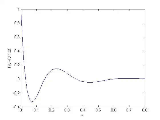
1. Use MATLAB to plot ${\displaystyle F(5,-10;1;x)}$ near x=0 to show the local maximum (or maxima) in this region.

2. Show that ${\displaystyle F(5,-10;1;x)=(1-x)^{6}(1001x^{4}-1144x^{3}+396x^{2}-44x+1)}$

((1) pg. 64-9b)

The MATLAB code, shown below, will plot the hypergeometric function ${\displaystyle F(5,-10;1;x)}$ over the interval: ${\displaystyle 0\leq x\leq 0.8}$.

The plot of the hypergeometric function near x=0 reveals a local maximum of 0.1481 at x = 0.23.

The hypergeometric function ${\displaystyle F(5,-10;1;x)}$ can be expressed as ${\displaystyle \sum _{k=0}^{\infty }{\frac {(a)_{k}(b)_{k}}{(c)_{k}}}{\frac {x^{k}}{k!}}}$ using the Pochhammer Symbol

where   ${\displaystyle {\frac {(a)_{k}(b)_{k}}{(c)_{k}}}={\frac {a(a+1)(a+2)...(a+k-1)b(b+1)(b+2)...(b+k-1)}{c(c+1)(c+2)...(c+k-1)}}}$

(Eq. 5.10.1)

Here ${\displaystyle a=5}$, ${\displaystyle b=-10}$ and ${\displaystyle c=1}$.

The hypergeometric series represented by ${\displaystyle F(5,-10;1;x)}$ terminates after the 11th term because the constant b = -10. This is because starting with the 12th term in the series the factor ${\displaystyle (b+k-1)}$ appears in the numerator.

For the 12th term in the series k = 11, so ${\displaystyle (-10+11-1)=0}$

The hypergeometric series represented by the function ${\displaystyle F(5,-10;1;x)}$ can be written in expanded form:

${\displaystyle F(5,-10;1;x)=1-50x+675x^{2}-4200x^{3}+14700x^{4}-31752x^{5}+44100x^{6}-39600x^{7}+22275x^{8}-7150x^{9}+1001x^{10}}$

(Eq. 5.10.2)

If the expansion of ${\displaystyle (1-x)^{6}*(1001x^{4}-1144x^{3}+396x^{2}-44x+1)}$ agrees with (Eq. 5.10.2) then it is a valid representation of the hypergeometric function.

${\displaystyle (1-x)^{6}=1-6x+15x^{2}-20x^{3}+15x^{4}-6x^{5}+x^{6}}$

${\displaystyle (1-6x+15x^{2}-20x^{3}+15x^{4}-6x^{5}+x^{6})*(1001x^{4}-1144x^{3}+396x^{2}-44x+1)=}$

(Eq. 5.10.3)

${\displaystyle 1001x^{4}-6006x^{5}+15015x^{6}-20020x^{7}+15015x^{8}-6006x^{9}+1001^{10}}$

${\displaystyle -1144x^{3}+6864x^{4}-17160x^{5}+22880x^{6}-17160x^{7}+6864x^{8}-1144x^{9}}$

${\displaystyle 396x^{2}-2376x^{3}+5940x^{4}-7920x^{5}+5940x^{6}-2376x^{7}+396x^{8}}$

${\displaystyle -44x+264x^{2}-660x^{3}+880x^{4}-660x^{5}+264x^{6}-44x^{7}}$

${\displaystyle 1-6x+15x^{2}}$ ${\displaystyle -20x^{3}}$ ${\displaystyle +15x^{4}}$ ${\displaystyle -6x^{5}}$ ${\displaystyle +1x^{6}}$

Combining all like terms yields the following:

${\displaystyle 1-50x+675x^{2}-4200x^{3}+14700x^{4}-31752x^{5}+44100x^{6}-39600x^{7}+22275x^{8}-7150x^{9}+1001x^{10}}$

The expansion of (Eq. 5.10.3) agrees with the expanded form of the hypergeometric function (Eq. 5.10.2), which confirms that ((1) pg. 64-9b) is true.

${\displaystyle \int {\frac {dz}{az^{n}+b}}={\frac {1}{b}}z\ _{2}F_{1}\left(1,{\frac {1}{n}};1+{\frac {1}{n}};-a{\frac {z^{n}}{b}}\right)+k}$

(Eq.(1)p.63-9)

Where ${\displaystyle _{2}F_{1}(a_{1},a_{2};b_{1};x)}$ is a Hypergeometric Function.

Consider the integral in (3) Pg.63-8 and (Eq.(1)Pg.63-9)

${\displaystyle \int _{z(0)=0}^{z(t)}{\frac {dz}{az^{n}+b}}=-\int _{0}^{t}dt=-t}$

${\displaystyle \int {\frac {dz}{az^{n}+b}}={\frac {1}{b}}z\ _{2}F_{1}\left(1,{\frac {1}{n}};1+{\frac {1}{n}};-a{\frac {z^{n}}{b}}\right)+k}$

(Eq.5.11.1)

Let n=3, a=2 and b=10

For each value of time (t), solve for altitude z(t), plot z(t) vs t, and find the time when projectile returns to ground.

The given integral is a reduced form of the integral (3) Pg 63.8 which relates the mass of a projectile, the forces acting upon it when moving in air ( the air resistance, which is a function of its height in air, and its own weight) and the time taken for the projectile to reach the ground. Thus it represents a real world problem whose solution must actually exist.

We have been given the values of n, a and b. Substituting the values in (Eq.5.11.1), we get:

${\displaystyle \int {\frac {dz}{2z^{3}+10}}={\frac {1}{10}}z\ _{2}F_{1}\left(1,{\frac {1}{3}};1+{\frac {1}{3}};-2{\frac {z^{3}}{10}}\right)}$

${\displaystyle ={\frac {1}{10}}z\ _{2}F_{1}\left(1,{\frac {1}{3}};{\frac {4}{3}};{\frac {-2z^{3}}{10}}\right)}$

The solution of the above Hypergeometric function contains complex terms according to Wolfram Alpha ^[18] which does not seem to make sense as the function represents a real world problem with real numbers.

When expanded, this is a series that goes to infinity as there is no negative term in the hypergeometric function which will make one of the terms go to zero. This computation is beyond our ability. Hence the problem could not be solved.

1. Is (1)p.64-10 exact?

2. Is (1)p.64-10 in the power form of (3) p.21-1?

3. Verify that F(a,b;c;x) is indeed a solution of (1) p.64-10.

${\displaystyle \displaystyle x(1-x)y''+[c-(a+b+1)x]y'-aby=0}$

((1)p.64-10)

${\displaystyle \displaystyle G(x,y,y',y'')=g(x,y,p)+f(x,y,p)y''=0}$

((2)p.16-4)

${\displaystyle \displaystyle g(x,y,p):=\phi _{x}+\phi _{y}p}$

((3)p.16-4)

${\displaystyle \displaystyle f(x,y,p):=\phi _{p}}$

((4)p.16-4)

${\displaystyle \displaystyle p:=y'}$

((2)p.7-3)

${\displaystyle \displaystyle f_{xx}+2pf_{xy}+p^{2}f_{yy}=g_{xy}+pg_{yp}-g_{y}}$

((1)p.16-5)

${\displaystyle \displaystyle f_{xp}+pf_{yp}+2f_{y}=g_{pp}}$

((2)p.16-5)

${\displaystyle \displaystyle \alpha x^{r}y''+\beta x^{s}y'-\gamma x^{t}=0}$

((3)p.21-1)

1. In order for (1) p.64-10 to be exact, it must first be in the form of (2)p.16-4, with g and f defined in (3)-(4) p.16-4, as seen below.

${\displaystyle \displaystyle \underbrace {x(1-x)} _{\displaystyle \color {blue}{f(x,y,p)}}y''+\underbrace {[c-(a+b+1)x]y'-aby} _{\displaystyle \color {blue}{g(x,y,p)}}=0}$

(Eq. 12.1)

Therefore, the first exactness condition is satisfied.

In order to satisfy the second exactness condition, the following derivatives must be found.

${\displaystyle \displaystyle g=[c-(a+b+1)x]y'-aby=[c-(a+b+1)x]p-aby}$

(Eq. 12.2)

${\displaystyle \displaystyle g_{x}=-(a+b+1)p}$

(Eq. 12.3)

${\displaystyle \displaystyle g_{xp}=-(a+b+1)}$

(Eq. 12.4)

${\displaystyle \displaystyle g_{y}=-ab}$

(Eq. 12.5)

${\displaystyle \displaystyle g_{yp}=0}$

(Eq. 12.6)

${\displaystyle \displaystyle g_{p}=c-(a+b+1)x}$

(Eq. 12.7)

${\displaystyle \displaystyle g_{pp}=0}$

(Eq. 12.8)

${\displaystyle \displaystyle f=x(1-x)}$

(Eq. 12.9)

${\displaystyle \displaystyle f_{x}=x(-1)+1(1-x)=-x+1-x=1-2x}$

(Eq. 12.10)

${\displaystyle \displaystyle f_{xx}=-2}$

(Eq. 12.11)

${\displaystyle \displaystyle f_{xy}=0}$

(Eq. 12.12)

${\displaystyle \displaystyle f_{xp}=0}$

(Eq. 12.13)

${\displaystyle \displaystyle f_{y}=0}$

(Eq. 12.14)

${\displaystyle \displaystyle f_{yy}=0}$

(Eq. 12.15)

${\displaystyle \displaystyle f_{yp}=0}$

(Eq. 12.16)

By substituting into the 1st relation, (1) p.16-5:

${\displaystyle \displaystyle (-2)+2p(0)+p^{2}(0)=-(a+b+1)+p(0)-(-ab)}$

(Eq. 12.17)

${\displaystyle \displaystyle -2=-(a+b+1)+ab}$

(Eq. 12.18)

This is not true for all values of a and b, so the 1st relation is not valid.

By substituting into the 2nd relation, (2) p.16-5:

${\displaystyle \displaystyle (0)+p(0)+2(0)=(0)}$

(Eq. 12.19)

${\displaystyle \displaystyle 0=0}$

(Eq. 12.20)

This is true, so the 2nd relation is valid.

One of the relations is not valid, therefore the second exactness condition is not satisfied.

Hence, (1) p.64-10 is not exact.

2. The following equalities must be true for (1) p.64-10 to be in power form of (3) p.21-1.

${\displaystyle \displaystyle x(1-x)=x-x^{2}\neq \alpha x^{r}}$

(Eq. 12.21)

${\displaystyle \displaystyle c-(a+b+1)x\neq \beta x^{s}}$

(Eq. 12.22)

${\displaystyle \displaystyle -ab=-abx^{0}=\gamma x^{t},where\,\gamma =-ab;t=0}$

(Eq. 12.23)

Since there are no values of ${\displaystyle \displaystyle \alpha ,\beta ,r,s}$ that make these equalities true, then (1) p.64-10 is not in power form.

3. In order to verify that F(a,b;c;x) is a solution of (1) p.64-10, we select the example of ${\displaystyle \displaystyle y=F(1,1;1;x)\,since\,a,b,c\in \mathbb {R} }$.

${\displaystyle \displaystyle y=F(1,1;1;x)={\frac {1}{1-x}}}$

(Eq. 12.24)

Next, the first and second derivatives of y must be found.

${\displaystyle \displaystyle y'=-1*(1-x)^{-2}*-1={\frac {1}{(1-x)^{2}}}}$

(Eq. 12.25)

${\displaystyle \displaystyle y''=-2*(1-x)^{-3}*-1={\frac {2}{(1-x)^{3}}}}$

(Eq. 12.26)

Substituting into (1) p.64-10:

${\displaystyle \displaystyle x(1-x){\frac {2}{(1-x)^{3}}}+(1-3x){\frac {1}{(1-x)^{2}}}-{\frac {1}{1-x}}=0}$

(Eq. 12.27)

${\displaystyle \displaystyle {\frac {2x}{(1-x)^{2}}}+{\frac {1-3x}{(1-x)^{2}}}-{\frac {1-x}{(1-x)^{2}}}=0}$

(Eq. 12.28)

${\displaystyle \displaystyle {\frac {2x+1-3x-1+x}{(1-x)^{2}}}=0}$

(Eq. 12.29)

${\displaystyle \displaystyle {\frac {0}{(1-x)^{2}}}=0}$

(Eq. 12.30)

${\displaystyle \displaystyle 0=0}$

(Eq. 12.31)

This equation is valid, therefore, F(a,b;c;x) is a solution for (1) p.64-10.

Given

Legendre equation:

${\displaystyle \displaystyle G=(1-x^{2})y^{''}-2xy^{\prime }+n(n+1)y=0}$

(Eq. 5.13.1)

Hermite equation:

${\displaystyle \displaystyle y^{''}-2xy^{\prime }+2ny=0}$

(Eq. 5.13.2)

1. Verify the exactness of the Legendre (Eq. 5.13.1) and Hermite (Eq. 5.13.2) equations.

2. If Hermite equation is not exact, check whether it is in power form, and see whether it can be made exact using IFM with ${\displaystyle \displaystyle h(x,y)=x^{m}y^{n}}$.

3. The first few Hermite polynomials are:

${\displaystyle \displaystyle H_{0}(x)=1}$

${\displaystyle \displaystyle H_{1}(x)=2x}$

${\displaystyle \displaystyle H_{2}(x)=4x^{2}-2}$

Verify that these are homogeneous solutions to the Hermite differential equation (Eq. 5.13.2).

${\displaystyle \displaystyle p=:y'=:{\frac {dy}{dx}}}$

${\displaystyle \displaystyle f_{ij}={\frac {d^{2}f}{\partial i\partial j}}}$

To satisfy the first exactness condition, the Legendre equation (Eq. 5.13.1) should be of the form:

${\displaystyle \displaystyle G(x,y,y^{\prime },y^{''})=g(x,y,p)+f(x,y,p)y^{''}}$

(Eq. 5.13.3)

${\displaystyle \displaystyle G=\underbrace {(1-x^{2})} _{f(x,y,p)}y^{''}\underbrace {-2xy^{\prime }+n(n+1)y} _{g(x,y,p)}}$

Hence (Eq. 5.13.1) satisfies the first exactness condition.

The second exactness condition can be checked in two ways.

Method 1

The second exactness condition is satisfied if (Eq. 5.13.1) satisfies (Eq. 5.13.4) and (Eq. 5.13.5):

${\displaystyle \displaystyle f_{xx}+2pf_{xy}+p^{2}f_{yy}=g_{xp}+pg_{yp}-g_{y}}$

(Eq. 5.13.4)

${\displaystyle \displaystyle f_{xp}+pf_{yp}+2f_{y}=g_{pp}}$

(Eq. 5.13.5)

Computing derivatives,

${\displaystyle \displaystyle {\begin{aligned}&f_{xx}=-2\\&f_{xy}=0\\&f_{yy}=0\\&g_{xp}=-2\\&g_{yp}=0\\&g_{y}=n(n+1)\\&f_{xp}=0\\&f_{y}=0\\&f_{yp}=0\\&g_{pp}=0\end{aligned}}}$

Substituting these into (Eq. 5.13.4) and (Eq. 5.13.5),

(Eq. 5.13.4) ${\displaystyle \rightarrow -2+2p\cdot 0+p^{2}\cdot 0=-2+p\cdot 0-n(n+1)}$.

(Eq. 5.13.5) ${\displaystyle \rightarrow 0+p\cdot 0+2\cdot 0=0}$.

Hence, the second exactness condition is satisfied when ${\displaystyle \displaystyle n=0}$ or ${\displaystyle \displaystyle n=-1}$.

Method 2

The second exacness condition is met if (Eq. 5.13.1) satisfies:

${\displaystyle \displaystyle g_{0}-{\frac {dg_{1}}{dx}}+{\frac {d^{2}g_{2}}{dx^{2}}}=0}$

(Eq. 5.13.6)

where ${\displaystyle \displaystyle g_{i}:={\frac {\partial G}{\partial y^{(i)}}}}$

Computing the derivatives,

${\displaystyle \displaystyle {\begin{aligned}g_{0}&={\frac {\partial G}{\partial y^{(0)}}}=n(n+1)\\g_{1}&={\frac {\partial G}{\partial y^{(1)}}}=-2x\\g_{2}&={\frac {\partial G}{\partial y^{(2)}}}=1-x^{2}\\&{\frac {dg_{1}}{dx}}=-2\\&{\frac {d^{2}g_{2}}{dx^{2}}}=-2\end{aligned}}}$

Substituting these in (Eq. 5.13.6) yields,

${\displaystyle n(n+1)-(-2)-2=0}$

${\displaystyle n(n+1)=0}$

Again we see that the second exactness condition is satisfied when ${\displaystyle \displaystyle n=0}$ or ${\displaystyle \displaystyle n=-1}$.

To satisfy the first exactness condition, the Hermite equation (Eq. 5.13.2) should be of the form (Eq. 5.13.3):

${\displaystyle \displaystyle G=\underbrace {1} _{f(x,y,p)}\cdot y^{''}\underbrace {-2xy^{\prime }+2ny} _{g(x,y,p)}}$

Hence (Eq. 5.13.2) satisfies the first exactness condition.

The second exactness condition can be checked in two ways.

Method 1

The second exactness condition is satisfied if (Eq. 5.13.2) satisfies (Eq. 5.13.4) and (Eq. 5.13.5):

Computing the derivatives,

${\displaystyle \displaystyle {\begin{aligned}&f_{xx}=0\\&f_{xy}=0\\&f_{yy}=0\\&g_{xp}=-2\\&g_{yp}=0\\&g_{y}=2n\\&f_{xp}=0\\&f_{y}=0\\&f_{yp}=0\\&g_{pp}=0\end{aligned}}}$

Substituting these into (Eq. 5.13.4) and (Eq. 5.13.5),

(Eq. 5.13.4) ${\displaystyle \rightarrow 0+2p\cdot 0+p^{2}\cdot 0=-2+p\cdot 0-2n}$.

(Eq. 5.13.5) ${\displaystyle \rightarrow 0+p\cdot 0+2\cdot 0=0}$.

Hence, the second exactness condition is satisfied only when ${\displaystyle \displaystyle n=-1}$ This is a necessary condition.

Method 2

The second exacness condition is met if (Eq. 5.13.2) satisfies (Eq. 5.13.6).

Computing the derivatives,

${\displaystyle \displaystyle {\begin{aligned}g_{0}&={\frac {\partial G}{\partial y^{(0)}}}=2n\\g_{1}&={\frac {\partial G}{\partial y^{(1)}}}=-2x\\g_{2}&={\frac {\partial G}{\partial y^{(2)}}}=1\\&{\frac {dg_{1}}{dx}}=-2\\&{\frac {d^{2}g_{2}}{dx^{2}}}=0\end{aligned}}}$

Substituting these in (Eq. 5.13.6) yields,

${\displaystyle 2n-(-2)+0=0}$

${\displaystyle 2(n+1)=0}$

The second exactness condition is satisfied only when ${\displaystyle \displaystyle n=-1}$.

We have seen that the Hermite equation (Eq. 5.13.2) is not exact when ${\displaystyle \displaystyle n\neq -1}$.

The power form of L2-ODE-VC is

${\displaystyle \displaystyle \alpha x^{r}y''+\beta x^{s}y'+\gamma x^{t}y=0}$

(Eq. 5.13.7)

Comparing (Eq. 5.13.2) with (Eq. 5.13.7), we can see that the Hermite equation is of the power form with:

${\displaystyle \displaystyle \alpha =1;\beta =-2;\gamma =2n.}$

${\displaystyle \displaystyle r=0;s=1;t=0.}$

Hence, we can consider an integrating factor which is in power form, ${\displaystyle \displaystyle h(x,y)=x^{m}y^{n}}$

Replacing the 'n' term in (Eq. 5.13.2) with ${\displaystyle \alpha }$ to avoid confusion, we need to find ${\displaystyle m,n\in \mathbb {E} }$, such that the following N2-ODE is exact:

${\displaystyle \displaystyle x^{m}y^{n}(y''-2xy'+2\alpha y)=0}$

(Eq. 5.13.8)

The Hermite equation (Eq. 5.13.2) can be written as:

${\displaystyle \displaystyle G(x,y,y',y'')=\underbrace {2\alpha x^{m}y^{n+1}-2x^{m+1}y^{n}y'} _{g(x,y,p)}+\underbrace {x^{m}y^{n}} _{f(x,y,p)}y''}$

(Eq. 5.13.9)

(Eq. 5.13.9) should satisfy (Eq. 5.13.4) and (Eq. 5.13.5) to meet the second exactness condition.

Computing the derivatives,

${\displaystyle \displaystyle {\begin{aligned}&f_{xx}=m(m-1)x^{m-2}y^{n}\\&f_{xy}=mnx^{m-1}y^{n-1}\\&f_{yy}=n(n-1)x^{m}y^{n-2}\\&g_{xp}=-2(m+1)x^{m}y^{n}\\&g_{yp}=-2nx^{m+1}y^{n-1}\\&g_{y}=-2nx^{m+1}y^{n-1}p+2(n+1)\lambda x^{m}y^{n}\\&f_{xp}=0\\&f_{y}=nx^{m}y^{n-1}\\&f_{yp}=0\\&g_{pp}=0\end{aligned}}}$

Substituting the derivatives in (Eq. 5.13.4) and (Eq. 5.13.5),

(Eq. 5.13.4) ${\displaystyle \displaystyle \rightarrow \displaystyle m(m-1)x^{m-2}y^{n}+2p\cdot mnx^{m-1}y^{n-1}+p^{2}n(n-1)x^{m}y^{n-2}=-2(m+1)x^{m}y^{n}+p(-2nx^{m+1}y^{n-1})-2\alpha (n+1)x^{m}y^{n}+2nx^{m+1}y^{n-1}p}$

(Eq. 5.13.5) ${\displaystyle \displaystyle \rightarrow 0+p\cdot 0+2nx^{m}y^{n-1}=0}$

We can see that the second exactness condition can be satisfied only when ${\displaystyle \displaystyle n=0}$. When ${\displaystyle \displaystyle n=0}$,

${\displaystyle \displaystyle m(m-1)x^{m-2}=-2(m+1)x^{m}-2\alpha x^{m}}$.

Hence we can say

${\displaystyle \displaystyle m(m-1)=0}$

${\displaystyle \displaystyle m+1+\alpha =0}$

Therefore, ${\displaystyle \displaystyle m=1,\alpha =-2\,}$ is a solution.

Hence, (Eq. 5.13.2) can be made exact using the integrating factor ${\displaystyle \displaystyle h(x,y)=x}$

Case 1

${\displaystyle \displaystyle y=H_{0}(x)=1}$

${\displaystyle \displaystyle y'=H_{0}'(x)=0}$

${\displaystyle \displaystyle y''=H_{0}''(x)=0}$

Substituting in (Eq. 5.13.2), ${\displaystyle \displaystyle 0-2x\cdot 0+0\cdot 1=0}$

Case 2

${\displaystyle \displaystyle y=H_{1}(x)=2x}$

${\displaystyle \displaystyle y'=H_{1}'(x)=2}$

${\displaystyle \displaystyle y''=H_{1}''(x)=0}$

Substituting in (Eq. 5.13.2), ${\displaystyle \displaystyle 0-2x\cdot 2+2\cdot 2x=0}$

Case 3

${\displaystyle \displaystyle y=H_{2}(x)=4x^{2}-2}$

${\displaystyle \displaystyle y'=H_{2}'(x)=8x}$

${\displaystyle \displaystyle y''=H_{2}''(x)=8}$

Substituting in (Eq. 5.13.2), ${\displaystyle \displaystyle 8-2x\cdot 8x+4\cdot (4x^{2}-2)=0}$

Hence the given first three Hermite polynomials are homogeneous solutions of the Hermite equation.

Given

${\displaystyle \displaystyle X^{(4)}-K^{4}X=0}$

(Eq. 5.14.1)

${\displaystyle \displaystyle X(x)=e^{(rx)}}$

(Eq. 5.14.2)

Where

${\displaystyle \displaystyle r_{1,2}=\pm K}$

${\displaystyle \displaystyle r_{3,4}=\pm i\,K}$

Find expressions for ${\displaystyle \displaystyle X(x)}$ in terms of ${\displaystyle \displaystyle \cos Kx,\sin Kx,\cosh Kx,\sinh kh}$

By definition,

${\displaystyle \displaystyle e^{iKx}=\cos Kx+i\sin Kx}$ and

${\displaystyle \displaystyle e^{Kx}=\cosh Kx+\sinh Kx}$

Hence, (Eq. 5.14.2) can be written as:

${\displaystyle \displaystyle X(x)=C_{1}(\cosh Kx\ +\sinh Kx)+C_{2}(\cosh Kx\ -\sinh Kx)+C_{3}(\cos Kx+i\sin Kx)+C_{4}(\cos Kx-i\sin Kx)}$

${\displaystyle \displaystyle \rightarrow X(x)=c_{1}\cosh Kx\ +c_{2}\sinh Kx+c_{3}\cos Kx+c_{4}\sin Kx}$

(Eq. 5.14.3)

where,

${\displaystyle \displaystyle c_{1}=C_{1}+C_{2}}$

${\displaystyle \displaystyle c_{2}=C_{1}-C_{2}}$

${\displaystyle \displaystyle c_{3}=C_{3}+C_{4}}$

${\displaystyle \displaystyle c_{4}=i(C_{3}-C_{4})}$

Hence, (Eq. 5.14.3) is a generic expression for X(x).

Problem Contribution
Problem number	Solved by	Typed by	Proofread by
R5.1	Ramchandra, Mohammed	Ramchandra	Linghan
R5.2	Amrith, Fabian	Amrith	Ramchandra
R5.3	Linghan, Sarah	Linghan	Amrith
R5.4	Linghan, Rahul	Linghan	Fabian
R*5.5	Rahul, Mohammed, Fabian	Rahul	Amrith
R*5.6	Ramchandra, Amrith, Linghan	Ramchandra	Fabian
R*5.7	Linghan, Sarah, Mohammed	Linghan, Ramchandra	Ramchandra
R*5.8	Mohammed, Amrith	Mohammed	Rahul
R5.9	Ramchandra, Rahul	Ramchandra	Sarah
R5.10	Fabian, Amrith	Fabian	Ramchandra
R5.11	Fabian, Ramchandra, Amrith	Ramchandra	----
R5.12	Sarah, Fabian, Mohammed	Sarah	Amrith
R*5.13	Rahul, Ramchandra, Sarah	Rahul	Mohammed
R*5.14	Rahul, Sarah, Linghan	Rahul	Mohammed

1. ↑ Lecture Notes Setion 20 Pg. 20-2b
2. ↑ Lecture Notes Section 20 Pg 20-2b
3. ↑ Lecture Notes Section 20 Pg 20-1
4. ↑ Euler Formula
5. ↑ Lecture Notes Section 21 Pg 21-5
6. ↑ Lecture Notes Section 21 Pg 21-4
7. ↑ Lecture Notes Section 21 Pg 21-5
8. ↑ Lecture Notes Section 21 Pg 21-4
9. ↑ Lecture Notes Section 21 Pg 21-6
10. ↑ Lecture Notes Section 16
11. ↑ Lecture Notes Section 22 Pg 22-4
12. ↑ Lecture Notes Section 22 Pg 22-6
13. ↑ Lecture Notes Section 64 Pg 64-7b
14. ↑ Taylor Series Wiki
15. ↑ Lecture Notes Section 64 Pg 64-4
16. ↑ Lecture Notes Section 64 Pg 64-9b
17. ↑ Lecture Notes Section 64 Pg. 64-9b
18. ↑ Wolfram Alpha's Solution to Hypergeometric Function
19. ↑ Lecture Notes Section 27 Pg 27-1, 27-2
20. ↑ Lecture Notes Section 30 Pg 30-3